Phenology on the edge

Hi everyone! My name is Ian and I am a new PhD student with Josh. As part of our first term, we had to take Josh’s course “Geospatial Data Mining,” in which we learned how to find, manipulate, and analyze satellite images. Our main goal of the course was a project that we designed using some of the geospatial techniques we learned in class. In other years the projects were turned into papers, so I was excited for the possibilities this project had.

Being a field ecologist by training, I’ve been learning about edge effects for years. Specifically, I’ve been told that edge effects are bad, and can be detrimental for forests where fragmentation constantly leads to a cycle of degradation. Early in Josh’s class I discovered it was easy to calculate the normalized difference vegetation index (NDVI), which gives a greenness index (0-1) of the vegetation; in short, healthy forests are much greener (>0.66) while degraded forests are less so (<0.4). Given what we know about edge effects and our focus on spatial autocorrelation (closer things in space are more alike each other), I wondered: is there an edge effect on forest phenology?

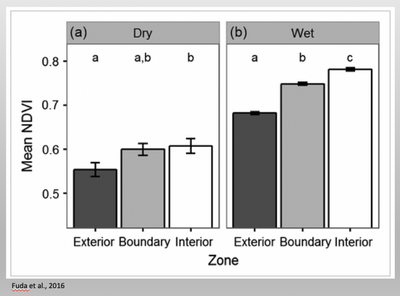
What I thought was a simple question turned out to have little proven foundation. There was not the breadth of literature I had hoped, but I did find a couple papers that convinced me I was on to something. Namely, Fuda et al. (2016) revealed this exact trend in Uganda, while Melaas et al. (2016) found that urban trees in Boston had longer growing seasons than non-urban trees. While I didn’t know how the Uganda study would transfer for temperate forests, the Boston study seemed like a direct match. In my view, urban trees are all mini-edges, thus a definitive study showing longer growing seasons seemed a different way of saying that edge trees have different phenology by proxy, and would consequently have different NDVI than, say, a forest interior.

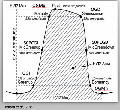
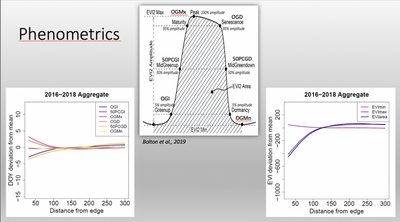
In order to establish a robust preliminary study, Josh suggested I use newly available moderate resolution phenometrics from 2016-2018 along with NDVI. These data are land surface phenology measurements taken from Harmonized Landsat-Sentinel (HLS) image time series. The HLS data are created from the fusion of Landsat 8 and Sentinel 2A/B satellites, and offer consistent, 30 m, multispectral measurements with a revisit time of around 3 days. Time series of the enhanced vegetation index (EVI) from HLS are processed to retrieve the timing of threshold crossing dates and related information such as integrated EVI (see schematic from Bolton et al., 2019). The specific measurements I obtained from HLS product were the minimum, maximum, and seasonally-integrated EVI, and the dates of the 5%, 50%, and 95% EVI amplitude crossing dates in spring and autumn (EVImin, EVImax, EVIarea, OGI, 50PCGI, OGMx, OGD, 50PCGD, and OGMn).

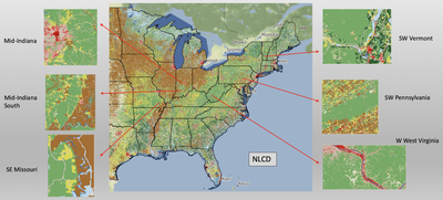
Once I identified my study sites, the project was an exercise in hurry up and wait. Sites were determined from the National Land Cover Database (NLCD) for areas that had forest to non-forest edges, including a variety of edge types and direction. Though most of the subsequent methodology was a lot of “oh I have an idea!” … “what did I do for the last 3 hours?”, it can be summed up like this: after masking the forest areas, I created a distance raster that showed the distance from every non-forest pixel to every forest pixel. Using that raster as my base, I then tabulated those distances with the days of year for each 30 m pixel from HLS. Admittedly, visualizing the results stopped me cold. While some plots showed clear trends from the edge to the interior, others showed no trends at all, or at least, not what I’d expect. I decided to push ahead with NDVI regardless.

NDVI was extracted in a similar way to the phenometrics but with some differences. Since NDVI is a daily metric as opposed to the annual HLS, I chose a day close to but after each site’s maximum greenness (OGMx) for each year. Afterwards, the methods were the same save for an extra resampling step since some Sentinel 2 image bands have a resolution of 10 m, allowing for a more fine-scale look at a possible gradient over distances.

Upon aggregating over all years and sites, the results showed what I had been hoping to see: a definite gradient in all variables from the forest edge to the interior. Despite some clear outliers, the main takeaways were that compared to the interior, the edge has

• An earlier green-up (OGI)
• A faster green-down (driven by a later senescence (OGD) and earlier mid-green-down (50PCGD)
• A larger growing season (potentially evidenced by earlier OGI [green-up] and smaller EVIarea at edge)
• Higher base productivity, but lower overall productivity (seen from a higher EVImin at edge, but lower EVImax and EVI area)
• A lower NDVI

Other than my results holding true to my original hypothesis, I was most surprised by how evident these effects were seen. In ecology we are usually told that edge effects are felt only within the first 100 m or so for forests, and this can sometimes be as low as 10 m when you’re talking about tropical rainforest to savannah edges. However, most of the variables showed trends lasting at least 100 m into the forest, and often further.

So why is this important? Forest fragmentation is occurring everywhere, and as this deforestation happens, we lose that much more ability to sequester carbon from the atmosphere. Although prevailing thought is these edges are net carbon sources, some studies (Reinnman and Hutyra, 2017; Smith et al., 2018) are showing the edges are actually carbon sinks, but ultimately they are still more susceptible to edge effects. In short, we don’t know the full dynamics resulting from fragmentation, but being able to definitively identify a gradient of phenometrics and NDVI can help give clues for further research. For example, using a gradient we would be able to more effectively model carbon fluxes and the global carbon balance. In addition, this would give a better estimate of future directions based on both climate scenarios and the degree of further deforestation / fragmentation.

In my view, ideal next steps would involve potentially running a mixed effects model with climate variables, topography, solar insolation (direction of edge), edge type, and species at each edge to see what the main drivers are of the individual site-year effects we see. We ultimately know that spring is arriving earlier in several regions across the US, but I’m now fascinated wondering if this earlier arrival is being driven more by the increasing number of edges (that get earlier green-up) than general climate change over interior forest. I’m not sure I’m completely right about that hypothesis, but then again, I thought I was wrong about this one.

References

Bolton et al., 2019 (in review).

Fuda, R.K., Ryan, S.J., Cohen, J.B., Hartter, J., Frair, J.L., 2016. Assessing impacts to primary productivity at the park edge in Murchison Falls Conservation Area, Uganda. Ecosphere 7, e01486. https://doi.org/10.1002/ecs2.1486

Melaas, E.K., Wang, J.A., Miller, D.L., Friedl, M.A., 2016. Interactions between urban vegetation and surface urban heat islands: a case study in the Boston metropolitan region. Environ. Res. Lett. 11, 054020. https://doi.org/10.1088/1748-9326/11/5/054020

Reinmann, A.B., Hutyra, L.R., 2017. Edge effects enhance carbon uptake and its vulnerability to climate change in temperate broadleaf forests. Proc Natl Acad Sci USA 114, 107–112. https://doi.org/10.1073/pnas.1612369114

Smith, I.A., Hutyra, L.R., Reinmann, A.B., Marrs, J.K., Thompson, J.R., 2018. Piecing together the fragments: elucidating edge effects on forest carbon dynamics. Frontiers in Ecology and the Environment 16, 213–221. https://doi.org/10.1002/fee.1793